In previous work (Fitzgibbon, Dowe, and Allison, 2002b,a) we have presented the Message from Monte Carlo (MMC) methodology, a general methodology for performing minimum message length inference using posterior sampling and Monte Carlo integration. In this section we describe the basic elements of the Message from Monte Carlo methodology. These elements will be used in the algorithms given in the following sections.
The basic idea is to partition a sample from the posterior distribution of the parameters into uncertainty regions representing entries in the MML instantaneous codebook. Each region has a point estimate which characterizes the models in the region. The point estimate is chosen as the minimum prior expected Kullback-Leibler distance estimate over the region. The regions are chosen so that the models contained within a region are similar in likelihood and Kullback-Leibler distance (to the point estimate).
Each region also has an associated message length which can be considered as the negative logarithm of the weight attributed to the region. The posterior epitome is the set of point estimates (one for each region) weighted by the antilog of the negative message length.
The message length approximation that is generally used in MMC is Dowe's MMLD minimum message length approximation (Fitzgibbon, Dowe, and
Allison, 2002a, section 2.4). Given an uncertainty region of the parameter space, ![]() , prior distribution,
, prior distribution, ![]() , and likelihood function,
, and likelihood function,
![]() , the message length of the region,
, the message length of the region, ![]() , is
, is
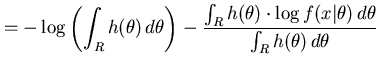
The MMLD message length equation can be seen to contain two terms. The first term is the negative logarithm of the integral of the prior over the region. It approximates the length of the first part of the MML message (i.e. ![]() ) from Equation 3. The second term is the prior expected negative logarithm of the likelihood function over the region. This approximates the MML message second part and is an average because we do not know the true estimate used in the first part. A shorter message length is to be preferred and involves a trade-off between the first and second terms. Consider a region growing down from the mode in a unimodal likelihood function. As the region grows the first term will decrease (as the integral of the prior increases) but the second term will increase (as the likelihood of the models added to the region decreases). The MMLD message length attempts to take into account the probability mass associated with the region surrounding a point estimate (rather than the point estimate's density for example).
) from Equation 3. The second term is the prior expected negative logarithm of the likelihood function over the region. This approximates the MML message second part and is an average because we do not know the true estimate used in the first part. A shorter message length is to be preferred and involves a trade-off between the first and second terms. Consider a region growing down from the mode in a unimodal likelihood function. As the region grows the first term will decrease (as the integral of the prior increases) but the second term will increase (as the likelihood of the models added to the region decreases). The MMLD message length attempts to take into account the probability mass associated with the region surrounding a point estimate (rather than the point estimate's density for example).
To calculate the MMLD message length we use importance sampling and Monte Carlo integration. We sample from the posterior distribution of the parameters
| (6) |
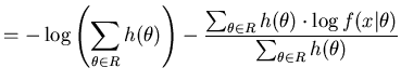
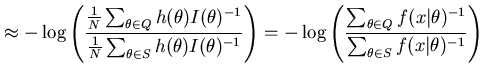
The second part is approximated using
These estimates allow the message length to be approximated for some ![]() . We now discuss how to select the
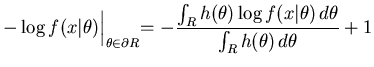
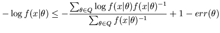
. We now discuss how to select the ![]() that minimises the message length. We first note that if we attempt to minimise Equation 4 we get the following boundary rule
that minimises the message length. We first note that if we attempt to minimise Equation 4 we get the following boundary rule
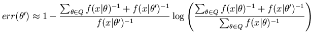
For the discrete version of MMLD (Equation 5) the boundary rule (Equation 9) is only an approximation and has the following error
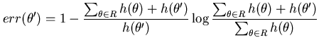 |
(10) |
Since the posterior sampling process has discretised the space we will need to include the ![]() term for both discrete and continuous parameter spaces. We can estimate the
term for both discrete and continuous parameter spaces. We can estimate the ![]() term using
term using
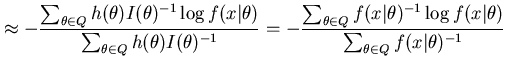
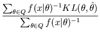
Due to the use of importance sampling the prior terms have cancelled and the estimate does not directly involve the prior. Intuitively we see that ![]() is largest when
is largest when ![]() is small and therefore
is small and therefore ![]() will have the largest effect when the region is initially being formed.
will have the largest effect when the region is initially being formed.
Selection of the optimal region is simple in the unimodal likelihood case since we can order the sample in descending order of likelihood, then start at the element with maximum likelihood and continue to grow the region accepting models into the region that pass the boundary rule test
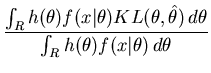
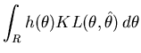
Once the region that minimises the message length is found we need to find a point estimate for the region. Staying true to the compact coding approach we use the minimum prior expected Kullback-Leibler distance estimate since this corresponds to the MMLA estimate (see (Fitzgibbon, Dowe, and
Allison, 2002a)[section 2.4.1]). This estimate represents a compromise between all of the models in the region and can be considered to be a characteristic model that summarises the region. The prior expected Kullback-Leibler (EKL) distance is
![$\displaystyle \hat{\theta} = argmin_{\hat{\theta} \in R} E_{h(\theta)} \left[ KL(\theta,\hat{\theta}) \right]$](img45.png) |
(15) |
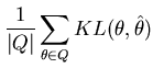
This estimate could be found by simulation (see, e.g. (Dowe, Baxter, Oliver, and Wallace, 1998) - note that they use the posterior expectation). It could also be found directly using Newton-Raphson type algorithms (as used in the next section). Both of these require that we know the parametric form of the estimate - making them less desireable for use with variable dimension posteriors. An alternative that does not have such a requirement is to find the element of ![]() that has the minimum EKL distance.
This algorithm was used in the MMC algorithm from (Fitzgibbon, Dowe, and
Allison, 2002a)[section 3.4]. An exhaustive search (i.e.
that has the minimum EKL distance.
This algorithm was used in the MMC algorithm from (Fitzgibbon, Dowe, and
Allison, 2002a)[section 3.4]. An exhaustive search (i.e.
![$ argmin_{\hat{\theta} \in Q} E_{h(\theta)} \left[ KL(\theta,\hat{\theta}) \right]$](img46.png) ), using Equation 14, requires quadratic time in
), using Equation 14, requires quadratic time in ![]() although simple strategies can be employed to reduce this considerably.
although simple strategies can be employed to reduce this considerably.
In practice it is often beneficial to use the posterior expected Kullback-Leibler distance
![$\displaystyle E_{h(\theta)}\left[ KL(\theta,\hat{\theta}) \right]$](img39.png)
![$\displaystyle E_{h(\theta)f(x\vert\theta)}\left[ KL(\theta,\hat{\theta}) \right]$](img48.png)