Unimodal Likelihood Function

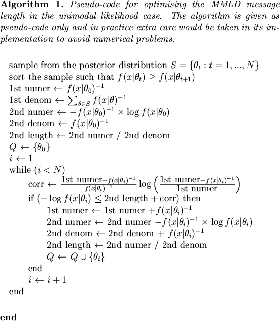
This section describes an MMC algorithm suitable for problems where the likelihood function is unimodal and of fixed dimension. A simple algorithm for finding the region with minimum message length is described, along with a Newton-Raphson algorithm for finding the point estimate.

For the unimodal likelihood function case the minimising MMLD region can be found using Algorithm 1. This algorithm is based on Algorithm 1 from (Fitzgibbon, Dowe, and Allison, 2002a, page 12) but has been modified to use the more accurate message length approximation described in the previous section. The algorithm is fast and efficient requiring a single pass through the sample. It produces a single region.

Choosing the point estimate can be more difficult than finding the region. For continuous parameter spaces of fixed dimension the Newton-Raphson algorithm is suitable. The Newton-Raphson method requires an initial estimate, $\theta^{(0)}$, for which we can use the element of the sample with maximum likelihood. Based on Equation 14, and using the notation $\hat{\theta} = (\hat{\vartheta_1},...,\hat{\vartheta_d})$, each iteration we update $\hat{\theta}^{(k+1)} = \hat{\theta}^{(k)} + d\hat{\theta}^{(k)}$ by solving the following linear system for $d\hat{\theta}^{(k)}$:

$$J \times d\hat{\theta}^{(k)} = -r$$ (18)

$$J = \left[ \begin{array}{ccc} \sum_{\theta \in Q} f(x\vert\theta)... ...\hat{\vartheta_d}} \Bigl\lvert_{\hat{\theta}^{(k)}} \right) \end{array} \right]$$ (19)

$$d\hat{\theta}^{(k)} = \left[ \begin{array}{c} d\hat{\vartheta_0}^... ...t{\vartheta_d}} \Bigl\lvert_{\hat{\theta}^{(k)}} \right) \\ \end{array} \right]$$ (20)

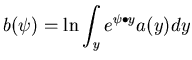
In the following ``Dog Shock Experiment" example we have used a numerical approximation for the second derivatives in $J$. In this example we also work in the canonical exponential form. The canonical exponential family (see (Bernardo and Smith, 1994)) of distributions have the following form

$$p(y\vert\psi) = a(y) e^{\psi \bullet y - b(\psi)} b(\psi) = \ln \int_y e^{\psi \bullet y} a(y) dy$$ (21)

Many commonly used distributions can be expressed as members of the exponential family and the Kullback-Leibler distance simplifies to

$$KL(\psi,\hat{\psi}) = -H(\psi) - E_{\psi}\left[ \log a(y) \right] + b(\hat{\psi}) - \hat{\psi} \bullet E_{\psi} y$$

$$= -b(\psi) + b(\hat{\psi}) + (\psi - \hat{\psi}) \bullet E_{\psi} y$$

$$= -b(\psi) + b(\hat{\psi}) + (\psi - \hat{\psi}) \bullet \nabla b(\psi)$$ (22)

We now illustrate the use of the unimodal MMC algorithm on two simple problems taken from the Bayesian Inference Using Gibbs Sampling (BUGS) (Gilks, Thomas, and Spiegelhalter, 1994) examples. The first is a parameter estimation problem involving a generalised linear model for binary data. The second is a parameter estimation and model selection problem involving a generalised linear model with three plausible link functions. WinBugs13 is used to do the sampling in both examples with a 1000 update burn-in and a final sample size of 10000.

Example: Dog Shock Experiment

In this example we apply the unimodal MMC algorithm to the dog shock learning model from Lindsey (1994). While this example is quite trivial, it is intended to illustrate how the unimodal MMC algorithm works. The sampler for this example can be found as BUGS example ``Dogs: loglinear model for binary data". Lindsey (1994) analysed the data from the Solomon-Wynne experiment on dogs. The experiment involved placing a dog in a box with a floor through which a non-lethal shock can be applied. The lights are turned out and a barrier raised. The dog has 10 seconds to jump the barrier and escape otherwise it will be shocked due to a voltage being applied to the floor. The data consists of 25 trials for 30 dogs. A learning model is fitted to the data where the probability that the $i^{\mbox{th}}$ dog receives a shock $\pi_k$ at trial $k$ is based on the number of times it has previously avoided being shocked $x_{ik}$ and the number of previous shocks $k-x_{ik}$ by the model

$$\pi_{ik} = \kappa^{x_{ik}} \times \upsilon^{k-x_{ik}}$$ (23)

or equivalently

$$\log(\pi_{ik}) = \alpha x_{ik} + \beta (k-x_{ik})$$ (24)

with $\alpha=\log(\kappa)$ and $\beta=\log(\upsilon)$. The important aspect of this model is that $\pi_{k}=\pi_{k-1} \kappa$ if the shock was avoided at trial $k-1$, or $\pi_{k}=\pi_{k-1} \upsilon$ if the shock was received at $k-1$. In other words the probability of a dog being shocked in the future changes by a factor of $\kappa$ each time a shock is avoided and by a factor of $\upsilon$ each time a shock occurs.

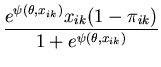
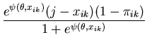
The unimodal MMC algorithm was run on the output from the BUGS program. The contents of the sample and the optimal region are shown in Figure 1. The message length of the region is 276.49 nits. The region contains 82 percent of the posterior probability. For this simple problem the message length and shape of the region is purely academic since there are no issues of model selection. We are more interested in the point estimate for the region. The following quantities are required for the Newton-Raphson point estimate algorithm (using notation from Equation 21)

$$\theta = (\alpha,\beta)$$ (25)

$$\psi(\theta,x_{ik}) = \log \frac{\pi_{ik}}{1 - \pi_{ik}}$$ (26)

$$a(y) = 1$$ (27)

$$b(\psi(\theta,x_{ik})) = \log (1+e^\pi_{ik})$$ (28)

$$\frac{\partial b(\psi(\theta,x_{ik}))}{\partial \psi} = \frac{e^{\psi(\theta,x_{ik})}}{1+e^{\psi(\theta,x_{ik})}}$$ (29)

$$\frac{\partial \psi(\theta,x_{ik})}{\partial \alpha} = x_{ik} (1 - \pi_{ik})$$ (30)

$$\frac{\partial \psi(\theta,x_{ik})}{\partial \beta} = (k-x_{ik}) (1 - \pi_{ik})$$ (31)

$$\frac{\partial b(\psi(\theta,x_{ik}))}{\partial \alpha} = \frac{e^{\psi(\theta,x_{ik})} x_{ik} (1 - \pi_{ik})}{1+e^{\psi(\theta,x_{ik})}}$$ (32)

$$\frac{\partial b(\psi(\theta,x_{ik}))}{\partial \beta} = \frac{e^{\psi(\theta,x_{ik})} (j-x_{ik}) (1 - \pi_{ik})}{1+e^{\psi(\theta,x_{ik})}}$$ (33)

The Newton-Raphson algorithm converged after six iterations to the estimates $\kappa=0.788$ and $\upsilon=0.924$. The estimate for $\upsilon$ corresponds with the posterior mean reported by BUGS and the maximum likelihood estimate from Lindsey (1994) to three decimal places. The estimate for $\kappa$ differs only in the third decimal place and lies above the mean and below the maximum likelihood estimate as can be seen in Figure 1.

The epitome for this example contains only a single entry with weight 1

$$\varepsilon = \{ ((\kappa=0.788,\upsilon=0.924),1) \}$$ (34)

Figure 1: Plot of the posterior sample (10,000 elements) for the dog shock data. The ellipse indicates the estimated MMLD boundary, $\partial R$, of the region, $R$. Parameter estimates: posterior mean=circle; maximum likelihood=diamond; MMC (minimum prior expected Kullback-Leibler distance)=square.

Example: Beetle Mortality Data

In this example we use the unimodal MMC algorithm to perform model selection for the BUGS example ``Beetles: logistic, probit and extreme value (log-log) model comparison". The example is based on an analysis by Dobson (1983) of binary dose-response data. In an experiment, beetles are exposed to carbon disulphide at eight different concentrations ($x_i$) and the number of beetles killed after 5 hours exposure is recorded.

Three different link functions for the proportion killed, $\pi_i$, at concentration $x_i$ are entertained

$$\pi_i = \frac{e^{\alpha + \beta x_i}}{1 + \alpha + \beta x_i}$$ Logit (35)

$$= \Phi (\alpha + \beta x_i)$$ Probit (36)

$$= 1 - e^{- e^{\alpha + \beta x_i}}$$ CLogLog (37)

Dobson (1983) used the log-likelihood ratio statistic to assess the three link functions for goodness of fit. The test showed that the extreme value log-log link function provided the best fit to the data. We ran the unimodal MMC algorithm on 10000 elements sampled from the posterior for each link function. The message lengths and corresponding normalised weights for each link function are given in Table 1. We see that MMC also provides strong support for the extreme value log-log link function, giving it a weight of 0.9. MMC gives more than twice the weight to the probit link compared to the logit link function. This is in contrast to the log-likelihood ratio statistic that gives only slightly more support for the probit model. From the table we can deduce that the peak of the probit model likelihood function contains more probability mass that that of the logit model. In other words the logit model gets less weight by MMC because the parameters lie in a region with slightly less posterior probability mass than the probit.

The epitome for this example contains entries corresponding to each link function

$$\varepsilon = \{ (\hat{\theta}_{logit},0.03), (\hat{\theta}_{probit},0.07),(\hat{\theta}_{cloglog},0.9) \}$$ (38)

Table 1: MMC analysis of beetle mortality data

Link	1st part length	2nd part length	Message length	Weight
Logit	2.098 nits	186.857 nits	188.956 nits	0.03
Probit	1.729 nits	186.219 nits	187.949 nits	0.07
CLogLog	2.145 nits	183.310 nits	185.456 nits	0.90